16 maart 2026

Frogwatch Dashboard Release 2026-03

The March 2026 release of the Frogwatch Dashboard includes new features, improvements, and bug fixes. Here's an overview of the most important changes.

New features

Public API

The Dashboard now has a public API that allows you to programmatically retrieve measurement data and upload indicator data. Read all about it in our detailed article about the API.

Trace events in overviews

Trace events are now displayed in the events table, histogram, and summary. This gives you a more complete picture of all measurement activity.

Tilt baseline configuration for x- and y-axis

It is now possible to set a baseline for both the x- and y-axis of tilt data. This allows you to more accurately monitor deviations relative to a reference position.

Firmware warnings

Organisation managers now receive a warning when devices have outdated firmware. The firmware update page also indicates per device whether the firmware is outdated.

Improvements

• Improved mobile layout - The top toolbar and cluster configuration page are now more usable on mobile devices.
• Clearer battery status - Battery status indication in the sensor status tables has been improved and made consistent between normal and mobile views.
• Chronological order in SBR B reports - Dates in the SBR B results table in reports are now in chronological order.

Bug fixes

• The temperature data y-axis on generic and deformation data plot pages is no longer out of view.
• Plot tooltips now show 2 decimals, and the y-axis range setting now supports up to 3 decimals.
• The zoom level of the interactive measuring points map is now restricted to supported zoom levels.
• Timestamps in exceedance plots on the alarms page are now displayed correctly.
• PDF reports now automatically get the correct .pdf file extension, preventing the browser from misinterpreting dots in the report title as a file extension.
• The sensor calibration document download dialog now works correctly.

12 maart 2026

New: Public API for Frogwatch Dashboard

The Frogwatch Dashboard now has a public API. This allows you to programmatically retrieve measurement data and process it in your own systems. In this article, we explain what the API is, who it's for, what you can do with it, and how to get started.

What is the Frogwatch Dashboard API?

The Frogwatch Dashboard API is a REST API that gives you direct access to measurement data stored in the Frogwatch Dashboard. The API offers two endpoints:

• Retrieve measurement data (GET) - Fetch timeseries data for a specific measuring point and data channel, such as vibration, displacement, tilt, or temperature.
• Upload indicator data (POST) - Upload indicator data to a measuring point of type 'indicator'.

The API is documented using the OpenAPI standard. Interactive documentation is available directly from the Dashboard, including example code in Python, Shell, Node.js, Ruby, and PHP.

Who is it for?

The API is intended for Frogwatch Dashboard users who want to integrate their measurement data into their own systems or workflows. For example:

• Engineering consultants who want to automatically incorporate vibration data into their own reporting systems or databases.
• Developers who want to build custom dashboards, analyses, or alerting based on Frogwatch data.
• Data analysts who want to periodically retrieve measurement data for further analysis in tools like Python, MATLAB, or Excel.
• Organizations that want to create API integrations between the Frogwatch Dashboard and other systems, such as their own monitoring platform or project management software.

Any user with an active Dashboard subscription can use the API.

What can you do with it?

With the GET endpoint, you can retrieve timeseries data per measuring point and data channel. Available data channels include:

• Vibration: vibration.x, vibration.y, vibration.z
• Velocity (SBR): sbra_speed.x, sbra_speed.y, sbra_speed.z
• Displacement: displacement
• Tilt: tilt.x, tilt.y
• Temperature: temperature
• Strain: strain
• And various other channels for acceleration, effective values, and traces

You specify a time period via the from and until parameters (in UTC). Optionally, you can enable or disable downsampling and set the sort order.

With the POST endpoint, you can upload your own indicator data to the Dashboard. This allows you to add external measurement values to a measuring point of type 'indicator', so you can view them alongside your Frogwatch data in the Dashboard.

Getting started

1. Create an API key

An organization manager can create an API key via the API keys page in the Dashboard. You use this key to authenticate your API requests.

2. Look up measuring point IDs

In the Dashboard, you'll find an overview of all your measuring points under API details in the project menu. This page shows their IDs, available data channels, and example URLs, making it easy to quickly find the right parameters for your API calls.

3. Retrieve data

Here's an example in Python to retrieve vibration data:

import requests

response = requests.get(
    "https://api.dashboard.frog.watch/api/v1/timeseries_data/{measuring_point_id}/vibration.x",
    headers={
        "authorization": "YOUR_API_KEY"
    },
    params={
        "from": "2026-03-01T00:00:00.000Z",
        "until": "2026-03-02T00:00:00.000Z"
    }
)

data = response.json()

# data["data"] contains a list of [timestamp, value] pairs
# data["metadata"] contains information about the measuring point and unit
for timestamp, value in data["data"]:
    print(f"{timestamp}: {value}")

Replace {measuring_point_id} with your measuring point's ID and YOUR_API_KEY with your API key. Both can be found in the Dashboard.

4. Interactive documentation

Click the API documentation button on the API details page to open the full, interactive API documentation. Here you can test API requests directly and view example code in the programming language of your choice.

Available for all Dashboard users

The API is available to all users with an active Frogwatch Dashboard subscription. If you have questions about the API or need help with integration, please contact us.

17 november 2025

Dashboard Tips and Tricks

Introduction

The Frogwatch Dashboard offers powerful capabilities for monitoring and analyzing vibration data. This is the first article in the series Tips & Tricks where we share useful tips and tricks to get the most out of your dashboard.

Tip 1: Use the search function to quickly navigate to projects and meters

Click on the magnifying glass in the top right or type / (slash) to activate the search function.

In this popup you can search by:

• Project name
• Meter name
• Meter ID

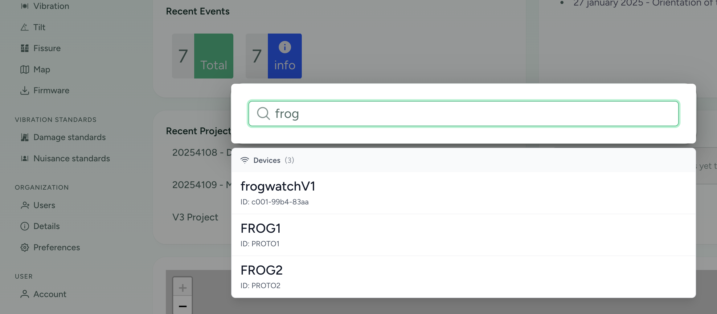
Use the arrow keys to browse through the list. Press enter to navigate to the page.

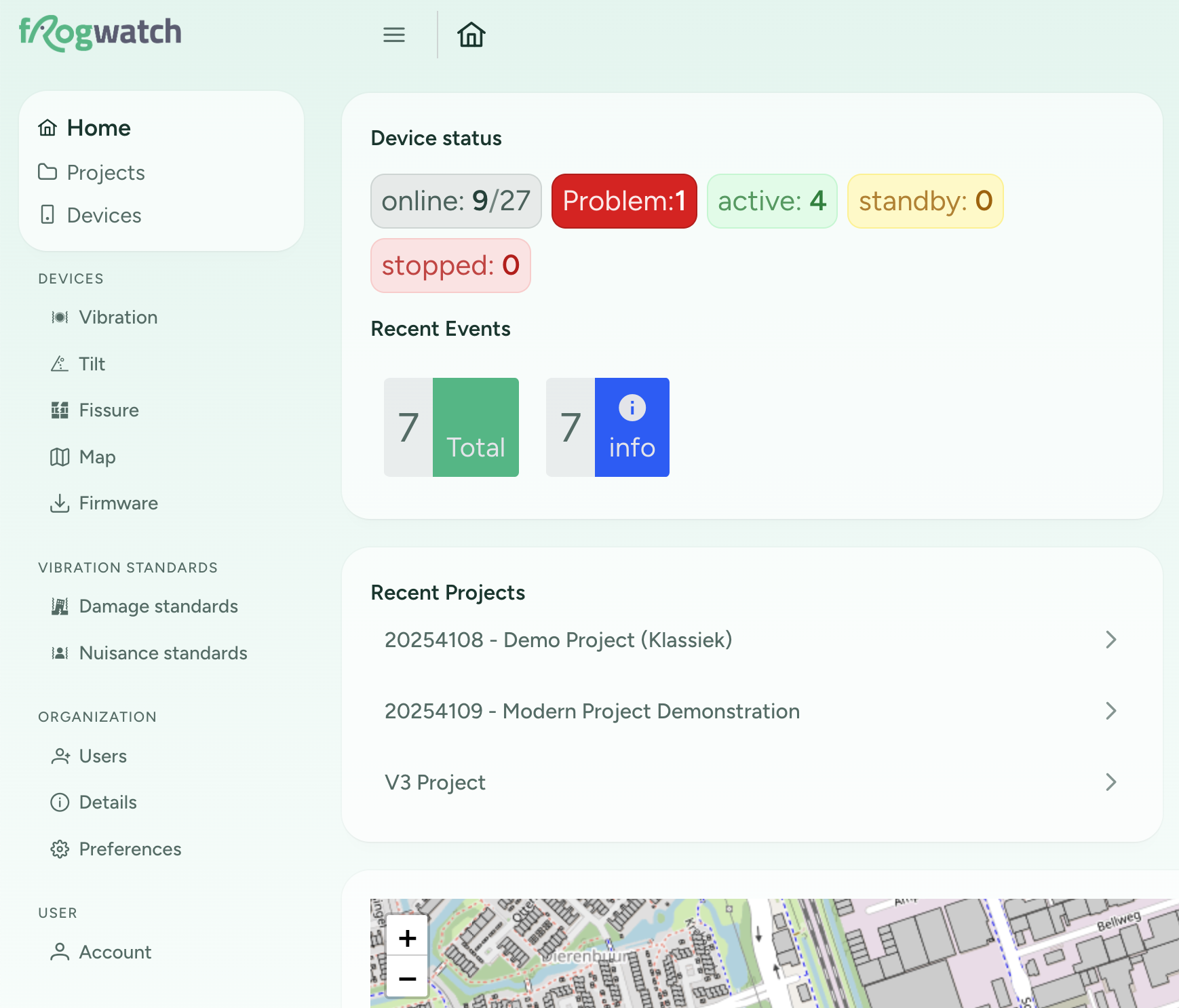
Tip 2: Recent Projects

On the "Home" page you will now find a list of recent projects. At the top is the project you most recently visited.

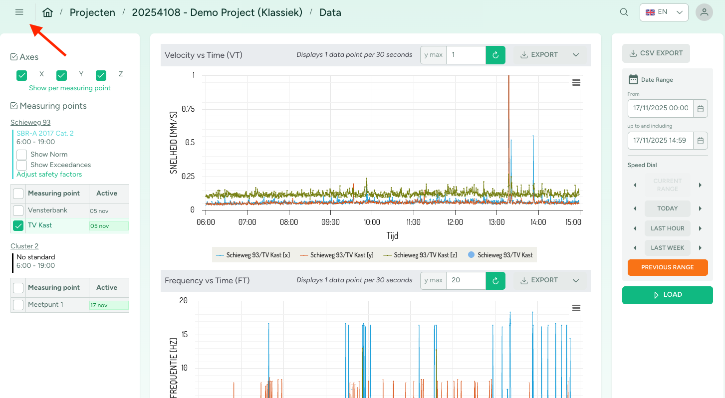
Tip 3: Hide the sidebar for more horizontal space

Click on the hamburger menu button to hide the sidebar. This will give you more horizontal space for your graphs.

10 november 2025

New Look for Frogwatch Dashboard

This month, Frogwatch Dashboard is getting a fresh new look. Why? With the introduction of the new Tilt and Crack measurements, we are taking the next step in our vision to make Frogwatch Dashboard the most user-friendly multi-sensor monitoring platform. To present data from different types of measurements clearly and intuitively, we needed a new structure and design. This update also allows us to make the website more suitable for mobile use. Together, these changes create a solid foundation for the future.

In this post, we highlight the main updates in the new look for existing users.

Main menu on the left side

In the new design, the main menu is now on the left side instead of at the top. The entire menu can be collapsed, so more space is available for your data. On smaller screens, such as mobile phones, the menu can be opened via the “hamburger” button.

Configure clusters on a single page

Previously, creating measurement points and linking devices to them was done on a different page from the measurement configuration. We have now combined these steps so that all cluster settings can be configured in one place, keeping everything clear and accessible on a single page.

Support for new measurement types

With support for new measurement types, we are also starting to phase out the older FrogwatchV1 vibration meters. For users who still use FrogwatchV1 meters, it will remain possible to do so within a Classic Project. When creating a new project, you can now choose between two options:

• Classic Project: a Frogwatch project as you know it, supporting both FrogwatchV1 and FrogwatchV2 vibration meters.
• Modern Project: The new Frogwatch project format that supports all the latest Frogwatch equipment but no longer supports FrogwatchV1 vibration meters.

If you only have FrogwatchV2 vibration meters, you will automatically get a Modern Project. All your existing projects will also be automatically upgraded.

New functionality will primarily be available in Modern Projects. Classic Projects will remain supported but will only receive minimal updates.

This Project Type choice is only visible if your organization still has FrogwatchV1 sensors.

More information coming soon

In upcoming articles, we will take a closer look at the new Dashboard features, explain the new concepts in more detail, and of course introduce the new Frogwatch devices: the Tilt Hub and the Fissure Hub.

24 maart 2025

Filtering of Vibration Data for SBR B Measurements

This is part 3 in the series "How does the Frogwatch Vibration Sensor work?". In this article, we discuss the signal processing applied in the Frogwatch Vibration Sensor when using the SBR B measurement method.

Signal processing flow chart

This flow chart schematically shows what happens to the measured sensor values for each of the axes (X, Y, and Z). Throughout the rest of the article, we refer to the P labels of the blocks in the flow chart. A part of the flowchart (up to and including P2) is the same as that of SBR A.

P1. Scaling to acceleration

The Frogwatch Vibration Sensor uses MEMS accelerometers to measure acceleration. The first step in the chain is scaling the raw sensor output to acceleration in mm/s2. For this scaling, we multiply the raw sensor data by a coefficient that is determined separately for each axis (X, Y, Z) through calibration against gravity.

After this, we have an unfiltered acceleration signal that still contains gravity. This means there is a 0 Hz component of about 9810 mm/s2 on one (or distributed over) of the axes. This is a very large signal compared to the typical SBR values we monitor for. For example, SBR Category 2 has threshold values between 5 and 20 mm/s2.

P2. Highpass filter

The highpass filter allows higher frequencies to pass and blocks low frequencies. In the Frogwatch Sensor, this filter serves two purposes:

1. Removing the gravity component. Since this is a 0 Hz signal, it is attenuated to the point of being negligible.
2. The low-frequency part of the prescribed SBR filter.

The gray area is prescribed by the SBR B guideline. The filter magnitude response must stay within this area to comply with the guidelines. This means there is some leeway. We have designed this filter so that it is suitable for both SBR A and SBR B.

P3. Lowpass filter

SBR guidelines specify that we are only interested in frequencies between 1 and 80 Hz for SBR B. Therefore, we use a lowpass filter to filter out frequencies above 80 Hz. This effectively makes the signal 'cleaner' because all high-frequency noise is filtered out.

In this figure, the transfer function of the lowpass filter is combined with that of the highpass filter. So, we are actually looking at the bandpass filter that meets the SBR B guidelines.

P5. SBR B - 5.6Hz low pass filter

When measuring according to the SBR B guideline, after the bandpass filter there is also a need for a first-order 5.6Hz weighting filter (SBR B section 9.2). Depending on whether the data is currently in the acceleration domain or the velocity domain, this filter should be either a lowpass or a highpass filter. If you measure with a geophone, your signal is by definition in the velocity domain, but also if you first integrate the measurement data, the guideline prescribes a 5.6Hz highpass filter. Since Frogwatch measures acceleration, we apply this filter:

At first, this feels counterintuitive: that we use either a lowpass or a highpass filter to measure the same thing. However, we can show mathematically why this is correct. We can rewrite the formula as:

where:

• $\frac{1}{2\pi f}$ is an integrator.
• $\frac{1}{\sqrt{1+(f_0/f{)}^2}}$ is a first-order highpass Butterworth filter (note that $f/f_0$ is inverted).

This confirms that the original filter is an integrator followed by a highpass filter.

For the full mathematical derivation, see this notebook. In the figure below, we also see how this filter combines with an ideal integrator. The drawn SBR B limits are purely for reference, to make it easier to compare with other filters we describe. We can therefore see that for SBR B, all acceleration signals are attenuated by at least 30dB. A large part of this comes from the implicit integrator.

P6. SBR B moving effective value filter

To ultimately calculate $V_{eff}$, SBR B 9.3 prescribes a moving effective value with a time constant of 125 milliseconds. In the guideline, this is defined with a complicated-looking integral:

Digitally, an integral does not exist, so we can implement this as a first-order IIR (Infinite Impulse Response) filter[1]:

where:

with $f_s=1000$ Hz (sampling frequency) and $\tau =0.125$ s (time constant).

This filter ensures that rapid changes are spread out over the time constant $\tau$, providing a good measure of the effective vibration strength over time.

[1] Signal Processing for Intelligent Sensor Systems - David Swanson 12.2

10 februari 2025

Filtering of Vibration Data for SBR A Measurements

This is part 2 in the series "How does the Frogwatch Vibration Sensor work?". In this article, we discuss the signal processing applied in the Frogwatch Vibration Sensor when configured for the Dutch SBR A measurement method.

Signal processing flow chart

This flow chart schematically shows what happens to the measured sensor values for each of the axes (X, Y, and Z). Throughout the rest of the article, we refer to the P labels of the blocks in the flow chart. The S branches represent the real-time data that is, for example, available via Triggered Traces.

P1. Scaling to acceleration

The Frogwatch Vibration Sensor uses MEMS accelerometers to measure acceleration. The acceleration signal is sampled at 1000 samples per second. The first step in the chain is scaling the raw sensor output to acceleration in mm/s2. For this scaling, we multiply the raw sensor data by a coefficient that is determined separately for each axis (X, Y, Z) through calibration against gravity.

After this, we have an unfiltered acceleration signal that still contains gravity. This means there is a 0 Hz component of about 9810 mm/s2 on one (or distributed over) of the axes. This is a very large signal compared to the typical SBR values we monitor for. For example, SBR Category 2 has threshold values between 5 and 20 mm/s2.

P2. Highpass filter

The highpass filter allows higher frequencies to pass and blocks low frequencies. In the Frogwatch Sensor, this filter serves two purposes:

1. Removing the gravity component. Since this is a 0 Hz signal, it is attenuated to the point of being negligible.
2. The low-frequency part of the prescribed SBR filter.

The gray area is prescribed by the SBR A guideline. The filter magnitude response must stay within this area to comply with the guidelines. This means there is some leeway. We have designed this filter so that it is suitable for both SBR A and SBR B.

P3. Lowpass filter

SBR guidelines specify that we are only interested in frequencies between 1 and 100 Hz for SBR A. Therefore, we use a lowpass filter to filter out frequencies above 100 Hz. This effectively makes the signal 'cleaner' because all high-frequency noise is filtered out.

In this figure, the transfer function of the lowpass filter is combined with that of the highpass filter. So, we are actually looking at the bandpass filter that meets the SBR A guidelines.

P4. Integrator

SBR standards are defined in the velocity domain and use mm/s as the unit. This originated because earlier generations of vibration sensors were based on geophone technology. A geophone measures velocity.

To be able to assess against the SBR standards and to allow the devices to be calibrated according to SBR guidelines, we integrate the acceleration data to velocity. Mathematically, an integrator is nothing more than a first-order lowpass filter. In the Laplace domain, we write this filter as

with $s=j\omega ,\omega =2\pi f$

The problem with an ideal integrator is that for frequencies $s<1$ the magnitude is amplified, e.g. $\frac{1}{s}=\frac{1}{0.01}=100$. So signals at frequency s=0.01 are amplified by a factor of 100, which would have very strange consequences.

To prevent this, we use a so-called leaky integrator. This ensures that the gain never exceeds 1.0.

In this figure, the blue line shows the transfer function of an ideal integrator. Both the green line and the dashed dark line are suitable leaky integrators. Within the spectrum of interest for SBR, they closely follow the ideal integrator. Below 1 Hz, they provide attenuation to keep the signal stable. The green line adds an extra 3dB of attenuation, which results in slightly less noise in the final result.

Calibration

This was, in broad terms, the data processing pipeline as implemented in the Frogwatch Vibration Sensor. The entire data processing pipeline as described here is ultimately tested during calibration. The calibration is performed in the velocity domain, and the measured values are read from the Frogwatch Dashboard. This way, we test the entire chain: sensors, filters, integrator, communication, database, and visualization.

In the figure above, you can see the result of a Frogwatch V2 Vibration Sensor on the shaker table at SONOR Calibration. The shaker table provides a constant acceleration at varying frequencies. In the graph below, you can clearly see the effect of filtering outside the range of 1-100Hz. There, a difference arises compared to the shaker table because our filters (as expected) attenuate the signal. The curves clearly show the attenuating effect of $\frac{1}{2\pi f}$ of the integrator.

27 januari 2025

Orientation of the Frogwatch Vibration Meter

Curious how the Frogwatch actually works? In this article series, we’ll walk through the entire measurement chain step by step and explain how Frogwatch arrives at the final measurement results.

Determining Orientation

The Frogwatch vibration sensor records vibrations in three directions: X, Y, and Z. Unlike many other devices, these directions are not fixed. Instead, the meter automatically detects how you have positioned it. How does that work?

The Frogwatch is based on a (MEMS) accelerometer. This type of sensor measures accelerations: besides vibrations, it also measures gravitational acceleration (gravity). Here on Earth, that’s a constant value of about 9.81 m/s².

By filtering out the effect of vibrations (i.e., averaging over a long enough period), we are left with a constant value in each of the three measurement directions, caused by gravity. The larger this value, the more that direction aligns with gravity: the direction with the largest value points downward!

Once the device knows which sensor axis points most towards gravity (downward), the X/Y/Z axes are assigned according to a fixed pattern:

• The vertical direction is called Z
• The direction along the wall is called Y
• The direction perpendicular to the wall is called X

Level or Not?

Because the Frogwatch Sensor knows the proportion of gravity measured on each axis, the system can use trigonometry to calculate how level the device is placed. Before the measurement starts, the meter performs a short self-test. If the meter is tilted by more than 3 degrees, a warning appears on the dashboard.

Why level the device?

Although it is not strictly necessary, we still recommend mounting the device as straight as possible. This ensures that:

• Vertical vibrations on the Z-axis: By mounting the device straight, vertical vibrations are measured as much as possible on the Z-axis. This prevents vibrations from being distributed over the other axes, which improves accuracy and interpretation.
• Uniformity in measurements: All Frogwatch sensors within a project measure in the same direction, which is essential for comparability.
• Reproducibility: Accurate repetition of measurements is possible, for example during zero measurements or long-term analyses.

How straight is straight enough?

In practice, "by eye" mounting is often sufficient. A deviation of more than 1 degree is easily noticeable visually, even without tools like a spirit level.